Data Ingestion Patterns
- The first question to ask is: How stale can this data be?
| Batch Ingestion | Streaming Ingestion |
| Collect data over a window (hourly, nightly, weekly), and process it all at onceExamples:Weekly Restaurant Payout ReportsDaily Dasher earnings summariesRetraining a ML model on historical order dataTools:AWS GlueAirflowFivetran | Every event is processed the moment it is emmitedExamples:Real-time orders status updatesSurge pricing calculationsFraud detectionTools:KafkaKinesis |
Kafka vs Kinesis: Kafka when you need control and scale; Kinesis when you want operational simplicity and are already AWS-native
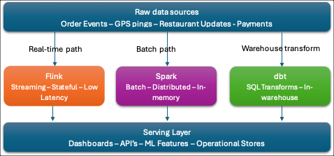
- Data Processing Frameworks
- Once data is ingested, something has to transform it.
- Think of this layer as the “computation engine” sitting between your raw data and your clean, queryable output.
| Apache Spark – large-scale batch processing – It runs distributed computations in-memory across a cluster, which makes it dramatically faster than old-school Hadoop MapReduce. – At DoorDash, Spark would power nightly jobs that aggregate millions of order records into dasher performance metrics, or backfill historical data when a schema changes. – It’s the right tool when your data is already at rest and you need to crunch a lot of it. |
| Apache Flink – Where Spark batch jobs run on a schedule, Flink runs continuously, processing events as they arrive with very low latency. – DoorDash would use Flink to compute rolling 15-minute ETA models fed by live GPS pings, or to detect anomalous order patterns (potential fraud) in real time. – Flink also supports “stateful” computations — it can remember context across events, which is critical for things like “has this dasher been idle for more than 20 minutes?” |
| dbt (data build tool) is different from both – it’s a transformation layer that runs SQL inside your warehouse. – It doesn’t move data; it transforms data that’s already landed. – Modeling layer where analysts and data engineers define clean, tested, documented tables. – DoorDash’s analytics team would use dbt to build the orders_daily, dasher_performance, and restaurant_metrics tables that power dashboards and reporting. – The key dbt concepts for interviews are models (SQL files), tests (assert that nulls/duplicates don’t exist), and lineage (the DAG of how tables depend on each other). |
Scalability Principles
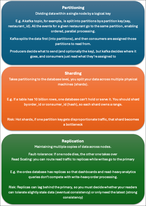
The CAP Theorem
- In a distributed system, you can only guarantee two of:
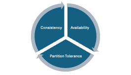
In the real-world, partition tolerance is non-negotiable (networks always fail sometimes).
Choose between:
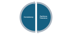
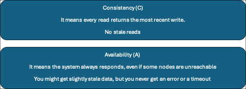
CP – Consistency but may be unavailable during partitions
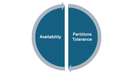
AP – Always available but may serves stale data
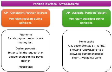
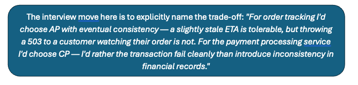
Eventual Consistency is the practical implementation of the AP choice. It means replicas will diverge temporarily during a partition, but given enough time without new writes, all replicas will converge to the same value. DoorDash’s restaurant menu cache is a perfect example — if the primary database is unreachable, the cache serves a slightly stale menu for a few seconds or minutes. Nobody gets hurt. The system catches up once connectivity is restored.
The Persistence Layer
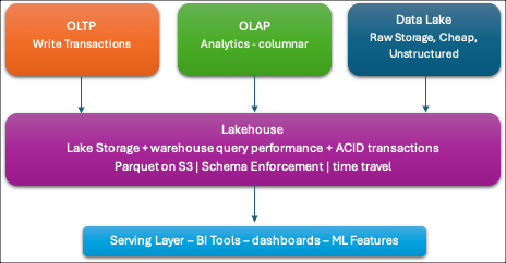
- OLTP (Online transaction Processing)
- High Volume
- Low latency reads and writes on small, precise rows
- Normalized (minimal data redundancy)
- Support ACID transactions
- Can handle thousands of writes per second
- MySQL, Postgress
- OLAP (Online Analytical Processing)
- Columnar storage (store data column-by-column rather than row-by-row)
- It makes aggregation blazingly fast but writes slow
- Snowflake, BigQuery, Redshift
- Data Lakes:
- Holds raw data
- Unstructured and semi-structured data at massive scale for low cost
- Querying this data is slow
- S2, GCS
- Lakehouses:
- Combines the best of both worlds
- Cheap lake storage with warehouse-quality query performance
- ACID transactions
- Store everything in the lake (parquet files on S3), but a metadata layer (Delta/Iceberg) tracks schema, file statistics, and versioning your query engine can efficiently prune files and run SQL at warehouse speeds
- Combines the best of both worlds
Example
| A GPS ping fires → ingested via Kafka (streaming ingestion) A Flink job consumes the event, updates the ETA model, and writes to a Redis cache for the customer app (real-time processing) The same event lands in S3 as a raw Parquet file (data lake) A nightly Spark job aggregates all GPS pings into dasher efficiency metrics (batch processing) dbt models transform those metrics into clean tables in Snowflake (warehouse transformation) A BI dashboard queries Snowflake to show ops teams which markets have dasher supply problems (OLAP serving) |
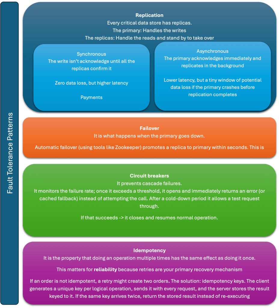
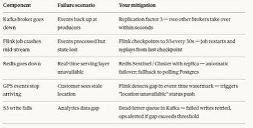
Scalability and Reliability
Reliability is about designing so that failures are contained, recoverable, and invisible to the user.
Knowing that failures will happen is step 1, designing around them is step 2.
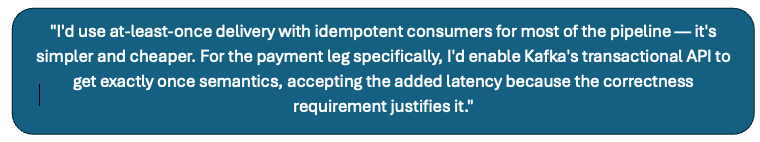
Delivery Guarantees
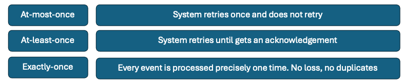
- If you are using, at-least-once, your consumers should be idempotent to handle duplicates
- If you are using, exactly-once, Kafka supports exactly-once semantics (EOS) through transactional producers and idempotent consumers; Flink has a checkpointing mechanism that achieves it end-to-end. The cost is latency and complexity.
Kafka over Kinesis (when not AWS-native):
“Kafka because we need sub-second latency, fine-grained partition control by market or order region, and long retention — Kinesis caps at 7 days by default and its fixed shard model makes rebalancing painful at 50K events/sec.”
Flink over Spark for real-time:
“Flink because it’s a true streaming engine — it processes events as they arrive with millisecond latency. Spark Structured Streaming micro-batches every few seconds, which violates our sub-3s SLA for the customer-facing update. Flink also supports stateful operations natively, which I need to join GPS pings with order records across event time.”
Redis over Postgres for serving:
“Redis because I’m serving 70K reads/second at sub-100ms latency. Postgres is disk-backed and can handle maybe 5–10K reads/second at that latency. Redis is in-memory and handles this trivially. The trade-off is durability — Redis can lose data on a crash — but that’s acceptable here because Postgres is the source of truth and Redis is a read cache.”
Parquet on S3:
“Parquet because it’s columnar and compressed — analytics queries that aggregate across millions of rows only read the columns they need, not full rows. At 86 GB/day compressed it’s also cost-effective on S3 compared to storing raw JSON.”
At 50K GPS events/second peak I need a distributed log as my ingestion layer. I’ll use Kafka — partitioned by market ID — because we need fine-grained partition control, sub-second latency, and long retention that Kinesis can’t match at this scale. From Kafka, two independent consumer groups fork the data.
The real-time path: a Flink job — not Spark, because I need true streaming with millisecond latency and stateful joins between GPS and order records. Flink writes the latest order state into Redis and publishes to a Redis channel. WebSocket servers subscribe and push updates to connected customers. Redis handles 70K reads/second at sub-100ms; Postgres couldn’t. Postgres remains the source of truth for the order state machine — every status transition is an ACID write there.
The analytics path: a second Flink consumer writes raw events as Parquet to S3 — columnar format, compressed roughly 10:1 to about 86 GB/day. dbt models in Snowflake transform that raw data into clean business tables. Looker queries Snowflake for ops dashboards.
For reliability: Kafka with replication factor 3, Flink checkpointing to S3 every 30 seconds for crash recovery, Redis Cluster for automatic failover, and a dead-letter queue for any events that fail to write to S3.
