Spark

Spark is a platform for cluster computing.

Spark lets you spread data and computations over clusters with multiple nodes (think of each node as a separate computer).
Splitting up your data makes it easier to work with very large datasets because each node only works with a small amount of data.
- As each node works on its own subset of the total data, it also carries out a part of the total calculations required, so that both data processing and computation are performed in parallel over the nodes in the cluster.
- It is a fact that parallel computation can make certain types of programming tasks much faster.

How to decide if you want to use Spark?

Is my data too big to work with on a single machine?
Can my calculations be easily parallelized?

Using Spark in Python

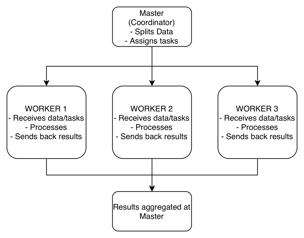
The cluster consists of multiple remote machines connected over a network. One machine acts as the master, and the others act as workers.

The master manages splitting up the data and the computations.
The master sends the workers data and calculations to run, and they send their results back to the master.

To create a connection, you only need to create an instance of the SparkContext class.

The class constructor takes a few optional arguments that allow you to specify the attributes of the cluster you’re connecting to.

DataFrames

Spark’s core data structure is the Resilient Distributed Dataset (RDD).

Low level object that let’s Spark work splitting data across multiple nodes in the cluster.
RDDs are hard to work with directly, so instead you can use Spark DataFrame abstraction built on top of RDDs.
The Spark DataFrame was designed to behave a lot like a SQL table (a table with variables in the columns and observations in the rows).
To start working with Spark DataFrames, you first have to create a SparkSession object from your SparkContext.
- You can think of the SparkContext as your connection to the cluster and the SparkSession as your interface with that connection

In the example below, you get to create a SparkSession, run a query, save the results to a pandas data frame, and print the head of the data frame.

			
# Import SparkSession from pyspark.sql
from pyspark.sql import SparkSession
# Create my_spark
my_spark = SparkSession.builder.getOrCreate()
# Print my_spark
print(my_spark)
# Don't change this query
query = "FROM flights SELECT * LIMIT 10"
# Get the first 10 rows of flights
flights10 = my_spark.sql(query)
# Show the results
flights10.show()
# Convert the results to a pandas DataFrame
pd_counts = flight_counts.toPandas()
# Print the head of pd_counts
print(pd_counts.head())

		

It is also possible to put a pandas DataFrame into a Spark cluster. The SparkSession class has a method for this as well.

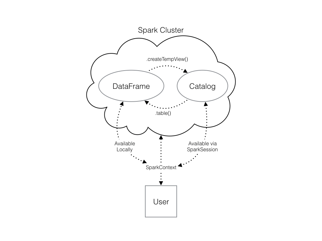
The .createDataFrame() method takes a pandas DataFrame and returns a Spark DataFrame. The output of this method is stored locally, not in the SparkSession catalog. This means that you can use all the Spark DataFrame methods on it, but you can’t access the data in other contexts.

You can’t use the .sql() method to reference the DataFrame since this will throw an error. You can save the data in a temp table, and use .createTempView() Spark DataFrame method to access the data. You can also use .createOrReplaceTempView() which creates a new temporary table if nothing was there before, or updates an existing table if one was already defined.

			
# Create pd_temp
pd_temp = pd.DataFrame(np.random.random(10))
# Create spark_temp from pd_temp
spark_temp = spark.createDataFrame(pd_temp)
# Examine the tables in the catalog
print(spark.catalog.listTables())
# Add spark_temp to the catalog
spark_temp.createOrReplaceTempView("temp")
# Examine the tables in the catalog again
print(spark.catalog.listTables())

		

You can also load data from external files:

			
# Don't change this file path
file_path = "/usr/local/share/datasets/airports.csv"
# Read in the airports data
airports = spark.read.csv(file_path, header=True)
# Show the data
airports.show()

		

Add a new column

			
# Create the DataFrame flights
flights = spark.table("flights")
# Show the head
flights.show()
# Add duration_hrs
flights = flights.withColumn("duration_hrs", flights.air_time/60)

		

Manipulating Data

Filter

			
# Filter flights by passing a string
long_flights1 = flights.filter("distance > 1000")
# Filter flights by passing a column of boolean values
long_flights2 = flights.filter(flights.distance > 1000)
# Print the data to check they're equal
long_flights1.show()
long_flights2.show()

		

Select

			
# Select the first set of columns
selected1 = flights.select("tailnum", "origin", "dest")
# Select the second set of columns
temp = flights.select(flights.origin, flights.dest, flights.carrier)
# Define first filter
filterA = flights.origin == "SEA"
# Define second filter
filterB = flights.dest == "PDX"
# Filter the data, first by filterA then by filterB
selected2 = temp.filter(filterA).filter(filterB)
# Define avg_speed
avg_speed = (flights.distance/(flights.air_time/60)).alias("avg_speed")
# Select the correct columns
speed1 = flights.select("origin", "dest", "tailnum", avg_speed)
# Create the same table using a SQL expression
speed2 = flights.selectExpr("origin", "dest", "tailnum", "distance/(air_time/60) as avg_speed")

		

Aggregating

			
# Find the shortest flight from PDX in terms of distance
flights.filter(flights.origin == "PDX").groupBy().min("distance").show()
# Find the longest flight from SEA in terms of air time
flights.filter(flights.origin == "SEA").groupBy().max("air_time").show()
# Average duration of Delta flights
flights.filter(flights.carrier == "DL").filter(flights.origin == "SEA").groupBy().avg("air_time").show()
# Total hours in the air
flights.withColumn("duration_hrs", flights.air_time/60).groupBy().sum("duration_hrs").show()

		

Grouping

			
# Group by tailnum
by_plane = flights.groupBy("tailnum")
# Number of flights each plane made
by_plane.count().show()
# Group by origin
by_origin = flights.groupBy("origin")
# Average duration of flights from PDX and SEA
by_origin.avg("air_time").show()

		

			
# Import pyspark.sql.functions as F
import pyspark.sql.functions as F
# Group by month and dest
by_month_dest = flights.groupBy("month", "dest")
# Average departure delay by month and destination
by_month_dest.avg("dep_delay").show()
# Standard deviation of departure delay
by_month_dest.agg(F.stddev("dep_delay")).show()

		

Joining

			
# Examine the data
airports.show()
# Rename the faa column
airports = airports.withColumnRenamed("faa", "dest")
# Join the DataFrames
flights_with_airports = flights.join(airports, on="dest", how="leftouter")
# Examine the new DataFrame
flights_with_airports.show()

		

Machine Learning Pipelines

At the core of the pyspark.ml module are the Transformer and Estimator classes.

Transformer classes have a .transform() method that takes a DataFrame and returns a new DataFrame; usually the original one with a new column appended.

Estimator classes all implement a .fit() method. These methods also take a DataFrame, but instead of returning another DataFrame they return a model object. This can be something like a StringIndexerModel for including categorical data saved as strings in your models, or a RandomForestModel that uses the random forest algorithm for classification or regression.

			
# Rename year column
planes = planes.withColumnRenamed("year", "plane_year")
# Join the DataFrames
model_data = flights.join(planes, on="tailnum", how="leftouter")
# Cast the columns to integers
model_data = model_data.withColumn("arr_delay", model_data.arr_delay.cast("integer"))
model_data = model_data.withColumn("air_time", model_data.air_time.cast("integer"))
model_data = model_data.withColumn("month", model_data.month.cast("integer"))
model_data = model_data.withColumn("plane_year", model_data.plane_year.cast("integer"))
# Create the column plane_age
model_data = model_data.withColumn("plane_age", model_data.year - model_data.plane_year)
# Create is_late
model_data = model_data.withColumn("is_late", model_data.arr_delay > 0)
# Convert to an integer
model_data = model_data.withColumn("label", model_data.is_late.cast("integer"))
# Remove missing values
model_data = model_data.filter("arr_delay is not NULL and dep_delay is not NULL and air_time is not NULL and plane_year is not NULL")
# Create a StringIndexer
carr_indexer = StringIndexer(inputCol="carrier", outputCol="carrier_index")
# Create a OneHotEncoder
carr_encoder = OneHotEncoder(inputCol="carrier_index", outputCol="carrier_fact")
# Create a StringIndexer
dest_indexer = StringIndexer(inputCol="dest", outputCol="dest_index")
# Create a OneHotEncoder
dest_encoder = OneHotEncoder(inputCol="dest_index", outputCol="dest_fact")
# Make a VectorAssembler
vec_assembler = VectorAssembler(inputCols=["month", "air_time", "carrier_fact", "dest_fact", "plane_age"], outputCol="features")
# Import Pipeline
from pyspark.ml import Pipeline
# Make the pipeline
flights_pipe = Pipeline(stages=[dest_indexer, dest_encoder, carr_indexer, carr_encoder, vec_assembler])
# Fit and transform the data
piped_data = flights_pipe.fit(model_data).transform(model_data)
# Split the data into training and test sets
training, test = piped_data.randomSplit([.6, .4])

		

Model Tuning and Selection

Logistic regression is very similar to a linear regression, but instead of predicting a numeric variable, it predicts the probability (between 0 and 1) of an event

To use this as a classification algorithm, all you have to do is assign a cutoff point to these probabilities. If the predicted probability is above the cutoff point, you classify that observation as a ‘yes’, if it’s below, you classify it as a ‘no’.

A hyperparameter is just a value in the model that’s not estimated from the data, but rather is supplied by the user to maximize performance.

You can tune your logistic regression model using a procedure called k-fold cross validation.

k-fold cross validation

It works by splitting the training data into a few different partitions. The exact number is up to you. Once the data is split up, one of the partitions is set aside, and the model is fit to the others. Then the error is measured against the held out partition. This is repeated for each of the partitions, so that every block of data is held out and used as a test set exactly once. Then the error on each of the partitions is averaged. This is called the cross validation error of the model, and is a good estimate of the actual error on the held out data.

The cross validation error is an estimate of the model’s error on the test set.

			
# Import the evaluation submodule
import pyspark.ml.evaluation as evals
# Create a BinaryClassificationEvaluator
evaluator = evals.BinaryClassificationEvaluator(metricName="areaUnderROC")
# Import the tuning submodule
import pyspark.ml.tuning as tune
# Create the parameter grid
grid = tune.ParamGridBuilder()
# Add the hyperparameter
grid = grid.addGrid(lr.regParam, np.arange(0, .1, .01))
grid = grid.addGrid(lr.elasticNetParam, [0, 1])
# Build the grid
grid = grid.build()
# Create the CrossValidator
cv = tune.CrossValidator(estimator=lr,
               estimatorParamMaps=grid,
               evaluator=evaluator
               )
# Call lr.fit()
best_lr = lr.fit(training)
# Print best_lr
print(best_lr)

		

AUC, or area under the curve is a common metric for binary classification algorithms. The curve is the ROC, or receiver operating curve.

The closer the AUC is to one (1), the better the model is.

			
# Use the model to predict the test set
test_results = best_lr.transform(test)
# Evaluate the predictions
print(evaluator.evaluate(test_results))